Options Volatility and Why Your Daily Commute Explains the Concept Better Than Finance Textbooks
Including homoscedasticity, realized volatility, and why 0DTE feels insane.
(TL;DR at end)
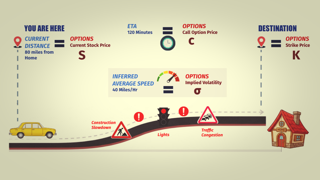
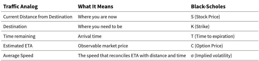
The Traffic Analogy
While sitting in traffic on the turnpike last week, my wife called to ask:
“When will you get home? You’ll get here before our friends arrive for dinner, right?”
I consulted Google Maps, and replied:
“Couple hours. But you know how the turnpike gets after 5.”
That single number (120 minutes) is not a fact of the world. It’s a model output!
I did not choose an average speed first. I committed to an ETA. And that ETA implied something important. I had assumed:
- a route,
- traffic conditions,
- estimated when I might arrive,
- with an average speed I expected I could maintain.
It struck me that I had just run a pricing model in my head. This is literally the entire Options market in one sentence.
Implied Volatility = The “Average Speed” Assumption
At 4:00 PM, when you say “120 minutes,” you assume something like:
“From here to home, I’m going to be on the I-95, which is fast (65 mph), the exit ramp, some lights (maybe wait an extra 10 minutes), finally city roads (30 mph). If all goes well, I get home by 6:00 PM, meaning I’ll be averaging something like 40 mph.”
That average speed is not what you’ll drive every second. But it’s the single number that reconciles:
- where you are now,
- where you’re going,
- into the ETA you quoted.
ETA = ƒ(distance, constraints, conditions)
You didn’t forecast the average speed. You backed it out from the ETA. That is exactly what implied volatility is.
Options markets observe the:
- current position (Spot Price of the underlying S)
- destination that matters (Strike K)
- time remaining to when you get home (Expiry T)
They then invert a pricing model which implies the average speed you’ll end up doing (Implied Volatility σ) that makes the ETA of 120 minutes (Call Price c) work.
Implied volatility is not a forecast. It’s the average variance rate implied by price, just like the average speed was implied by your ETA.
Note: Just because I used language like “you’re near home” doesn’t mean we’re taking a participant’s perspective. In option theory, the stock doesn’t belong to the call buyer or writer; they’re both simply exposed to the same path and have opposite payoffs on that path. In my driving analogy, the driver represents the underlying asset’s path; the call buyer and call writer are observers with opposite convex payoffs on the same journey.
Different Routes Mean Different Average Speeds = Volatility Smile
Let’s assume there’s multiple routes for which your ETA to home is the same:
- I-95 (interstate highway) – fastest when clear
- Garden State Parkway (state highway) – slower but predictable
- Toll road – different cost structure
- Downtown roads with traffic lights – high variance
Can you use the same “average speed” assumption for all of them? No!
Different options (different strikes) are like different routes: the payoff shape differs and so the “average speed” i.e., market-implied volatility needed to match the option price differs too. This is the volatility smile.
Black-Scholes assumes “one speed” for all routes. But markets know better!
Model Time vs. Clock Time (Where the Confusion Starts)
You keep checking your GPS while driving every 10 minutes and your ETA keeps changing, just like options are repriced continuously.
Each time you check, you’re not “updating” the old trip plan. You’re restarting the planning problem from where you are now.
Homoscedasticity of Volatility
Each repricing is a NEW model.
- All old estimates of ETA and volatility are now dead.
- Clock is reset to this moment.
- Remaining distance is remeasured,
- and the ETA you see implies the new single constant average speed from here on out to arrival.
What happened earlier on the road (smooth highways or traffic jams) are all behind you—they no longer enter the calculation.
Similarly, in option pricing:
- Time resets to zero in model time
- Variance is assumed constant from now to expiration
- Past returns or shocks are now irrelevant to the model.
This is why we say implied volatility is homoscedastic by construction inside the pricing model, even though realized volatility is not. And when you update the model, the new value of implied volatility is now homoscedastic inside the new pricing model. This also explains how implied volatility can jump intraday without violating homoscedasticity.
Homoscedasticity only holds inside each forward-looking pricing window, not across all time.
Volatility Clustering
Traffic systems have memory. Most days are calm until an accident, a storm, construction, etc. Think about driving after a major accident. One crash causes congestion, which causes more braking. The braking causes secondary accidents (because some driver was trying to hit ‘like’ on cat videos in a jam, then stupidly accelerated into another’s rear bumper). Rubbernecking slows traffic, lane closures persist and cleanup takes time.
As a result, speed variability stays high for a long time even after the initial event.
You get:
- Calm → Calm → Calm
- Shock → Chaos → More Chaos → Chaos → gradual normalization
That’s volatility clustering. In markets fear persists, liquidity dries up, correlations rise and trading becomes defensive. It works the other way as well. On clear days or off-peak hours, speed is smooth, predictable and stable. That’s the ‘low-volatility cluster’. Short-term variability can be huge, but over many commutes, traffic patterns revert to a long-run norm. Markets too behave similarly, with shocks spiking volatility, fear persisting and calm returning slowly.
This is why GARCH and regime-switching models exist.
Realized Volatility = What Actually Happened on the Road
Now consider your drive itself. You encountered:
- Open 8-lane highway stretches
- Stop-and-go lights
- Construction work with lower posted limits
- Sudden braking because the driver ahead of you was on TikTok
- Detours
When you look back at the trip data and measure how much your speed actually fluctuated, that’s Realized Volatility, which is:
- Backward-looking,
- Path-dependent,
- Shock-responsive,
- And clearly heteroscedastic.
Implied volatility is the plan, Realized Volatility is the trip log.
How the Greeks Work
Once you accept the driving analogy, the Greeks stop feeling abstract. It’s just a way to describe how your ETA reacts (sensitivity) as conditions change. The key variable is distance remaining, which maps directly to moneyness and time-to-expiry in options.
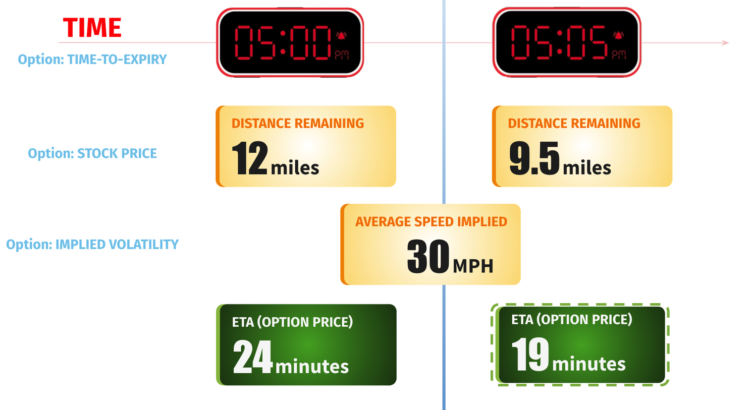
Theta: The Intuition Behind “Time Decay”
If nothing changes, except passage of time, how does my ETA change?
At 5:00 PM:
- Distance remaining = 12 miles
- With average speed = 30 mph
- ETA = 24 min.
Now it’s 5:05 PM. You’ve driven exactly as expected with no surprises along the same route and no change in assumed average speed. What happens to ETA?
ETA is now 19 minutes, not 24. So simply by letting time pass without surprises, your ETA shrinks. That is Theta.
Vega: Sensitivity to Uncertainty About the Trip
While driving, you get a push notification about a traffic or weather pattern forming 20 miles ahead on your route. There’s no observable delay yet, but you’re now more uncertain about the remainder of the drive.
Consequently:
- Your ETA is now less reliable
- The range of possible arrival times widens
- The implied “average speed” consistent with your ETA changes.
Vega measures how much your valuation changes when your uncertainty about the journey changes. It’s highest when there’s a lot of road ahead and collapses as arrival approaches.
That’s why long-dated options have high vega, and short-dated options have lower vega.
Vega is proportional to two things:
- How much future remains (time left) and,
- How much uncertainty can still flip the outcome
When you’re just minutes away from home:
- Weather later that night doesn’t matter to you anymore,
- Long-term traffic patterns are irrelevant,
- Only immediate movement counts.
Vega goes to zero as you approach option expiry.
Delta: Sensitivity to Distance
You’re 20 miles out, ETA is 40 minutes. What if you were 21 miles out? Maybe 42 minutes.
If your remaining distance changes a little, how much does ETA change? That’s Delta.
Example: Distance change = +1 mile and ETA change = +4 minutes.
If you’re far away from the destination, a small detour barely affects arrival time. At this point, Delta is low and stable. In options you can observe this in deep out-of-the-money options or deep-in-the-money options. Small price moves barely change option value (ETA).
If you’re close to the destination, you’re now on narrow local streets and small changes matter immediately.
Similarly, option Delta answers:
If the underlying moves a dollar right now, how much does the option price change?
Delta Hedging = Neutralizing Distance Errors
You have to get home and meet friends for dinner—e.g., you must arrive exactly at 6 PM. Being early or late is costly and distance measurement is noisy (GPS errors, detours, rerouting, etc.). That means you are exposed to distance uncertainty.
How do you neutralize distance risk? You’d dynamically adjust your route and speed to maintain that 6 PM promise regardless of where traffic puts you. Usually you add slack time, or leave earlier or choose a route with buffer zones or add an intermediate stop where timing can be adjusted.
Key idea:
Create a compensating mechanism so that if distance turns out to be slightly longer or shorter, your arrival time doesn’t change much.
That is delta hedging. You are removing first-order sensitivity to distance errors.
Delta hedging in options means:
- Long option + short underlying, OR
- Short option + long underlying
- Chosen such that ∂S has no effect.
But even after delta hedging, big surprises still hurt, sudden reroutes still matter and local road effects explode near arrival. This is because Delta itself changes.
Why Gamma Comes Out of Delta Changes
Now push the analogy a step further. Suppose you’re very far from home (100 miles). Small errors in distance (± 1 mile) barely change the ETA.
When you’re 2 miles from home on local streets with lights, moving one mile closer changes everything. As constraints tighten, and sensitivity itself changes, that’s curvature/convexity.
That essentially is Gamma. Delta gives you directional sensitivity while Gamma tells you how unstable that sensitivity is. Both Call and Put options are essentially long Gamma, meaning you have Gamma exposure.
Let’s say you carefully delta-hedged—i.e., you planned buffers to neutralize ETA sensitivity at the current distance. You’re now less than 5 minutes away from home. You’re on the highway and there’s one final exit to get off.
Small change happens: you missed the exit. Outcome explodes because you must now continue on the highway, drive several miles, find a U-turn, fight traffic back. ETA has jumped from 5 minutes to 20 minutes. Pure Gamma in action.
Or you’re literally pulling into your street and a school bus stops right in front of you. You fume behind the wheel while middle-schoolers literally drag their feet, chit-chatting and wasting time instead of getting off the bus quickly. “Please go”, you plead in your head. You can’t pass, can’t turn around, too late to detour. ETA jumped from seconds to minutes. This is 0DTE Gamma in its purest form.
0DTE = 0 Days To Expiry
Gamma Hedging = Redesigning the Trip Such That Mistakes Degrade Smoothly
You have alternatives. You could take an earlier exit and take slower surface roads for the final stretch. If you missed a turn, you only add +30 seconds and not +20 minutes. Or you could choose a grid with many parallel streets with multiple ways to get to the same block. Now a wrong turn is only a small correction. You replaced a cliff drop with a smooth slope.
Gamma-Theta Tradeoff
Hedging gamma is not free. You can either have a route that is:
- Fast, cheap but fragile, OR
- Smooth, forgiving and robust but slow.
Short a call or a put? You earn Theta but you are short Gamma. You’re the dude collecting rent for standing in front of a cliff. You eat risk.
So what do you do? You have to hedge the Gamma exposure. Here hedging Gamma means buying options, and that costs money. You’re paying for forgiveness with time.
Assume:
- SPX at 5000 and you are short near-dated ATM straddles
- You are short Gamma and earning Theta
To hedge, you buy:
- 4300 puts (far OTM downside)
- 5800 calls (far OTM upside)
These positions will bleed Theta for you, but that’s the price tag.
Example: How Domino’s Pizza Was Short Gamma and Long Theta

Domino’s in India runs a “30 minutes or free” offer. This is a digital barrier-style payoff.
If delivery time ≤ 30 mins: Customer pays full price.
If delivery time > 30 mins: Customer pays zero.
In options terms:
- Domino’s = Option seller
- Customer = Option buyer
- 30 minute cutoff = Strike / Barrier
- Delivery Time uncertainty = Volatility
- Free pizza if late = Convex payoff
Domino’s has a fixed upside (the pizza price), with a cliff-like downside (if delayed). This is textbook short Gamma. Small deviations around the cutoff (near 29 minutes) cause a large change in payoff ($X to $0). This is exactly the same thing as selling a short-dated option.
It’s great for the Indian pizza buyer who is essentially long Gamma. Any volatility shock like heavy rain, road closures or slowdowns due to things like political rallies, festivals all cause local bottlenecks that all work in your favor!
Domino’s hedged their short gamma position through operational strategies like:
- Route optimization and logistics
- Delivery radius restriction
- Limited delivery to high-probability zones
- Prep time efficiencies
- More drivers in peak time to reduce tail risk
All of which is basically decreasing vega exposure.
So What Did We Actually Learn?
Options theory doesn’t have to be understood solely through equations. They can be understood as contracts on uncertainty about a journey.
The mathematics may look intimidating, but the intuition? You’ve been doing it your whole life, every time you’ve tried to get somewhere on time.
TL;DR
Core Translation
| Traffic | Means | Options |
|---|---|---|
| ETA (120 min) | Observable arrival time | Option Price |
| Average Speed (40 mph) | Backs out from ETA | Implied Volatility |
| Current Distance | Where you are now | Stock Price (S) |
| Destination | Where you need to be | Strike Price (K) |
| Time Remaining | How much journey left | Time to Expiration (T) |
The Greeks in Traffic
Theta = ETA shrinks as time passes (even with no movement)
Vega = ETA changes when journey uncertainty increases (weather alerts)
Delta = How much ETA changes when distance changes
Gamma = How unstable Delta is (explodes near arrival i.e. if you miss your exit 2 min from home? +15 min penalty)
0DTE Gamma = School bus stops in front of you seconds from home (no time to adjust, outcome explodes)
Volatility Types
Implied Vol = Your planned “average speed” from here forward (homoscedastic inside each model)
Realized Vol = What actually happened on the road (stop-and-go, braking, construction—totally path-dependent)
Volatility Smile = Different routes need different average speeds to hit same ETA